
| 일 | 월 | 화 | 수 | 목 | 금 | 토 |
|---|---|---|---|---|---|---|
| 1 | ||||||
| 2 | 3 | 4 | 5 | 6 | 7 | 8 |
| 9 | 10 | 11 | 12 | 13 | 14 | 15 |
| 16 | 17 | 18 | 19 | 20 | 21 | 22 |
| 23 | 24 | 25 | 26 | 27 | 28 | 29 |
| 30 |
- 카트폴
- kaggle
- pandas
- GYM
- 리액트네이티브
- 사이드프로젝트
- JavaScript
- FirebaseV9
- python
- 데이터분석
- Reinforcement Learning
- 클론코딩
- ReactNative
- 조코딩
- selenium
- 강화학습
- redux
- Ros
- Instagrame clone
- App
- 딥러닝
- coding
- TeachagleMachine
- 머신러닝
- 강화학습 기초
- 전국국밥
- expo
- React
- 앱개발
- clone coding
- Today
- Total
qcoding
[LSTNET] 빌딩전력예측 딥러닝 본문
* 본 내용은 LSTNET이라는 Modeling Long- and Short-Term Temporal Patterns with Deep Neural Networks 논문에서 사용된 CNN+GRU의 Skip connection과 ARIMA 모델등에서 사용된 AR(Auto Regression)을 합친 것으로 시계열 예측에 사용되는 방법을 실습해 보았다.
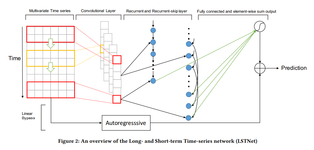
코드는 아래의 git-hup을 보고 model을 사용하였으며, 필요한 부분은 수정하여 사용하였다.
https://github.com/flaviagiammarino/lstnet-tensorflow
GitHub - flaviagiammarino/lstnet-tensorflow: TensorFlow implementation of LSTNet model for multivariate time series forecasting.
TensorFlow implementation of LSTNet model for multivariate time series forecasting. - GitHub - flaviagiammarino/lstnet-tensorflow: TensorFlow implementation of LSTNet model for multivariate time se...
github.com
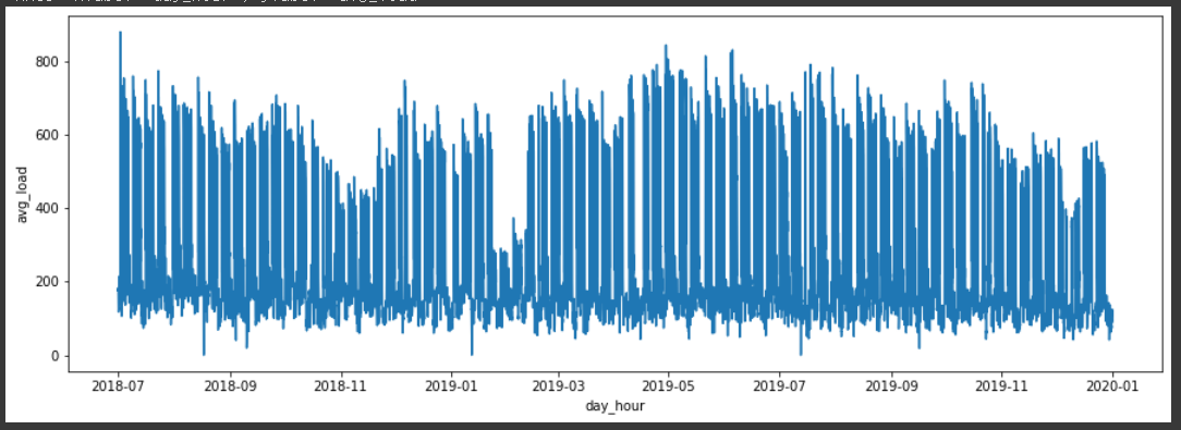
*앞의 블로그의 빌딩전력예측에서 사용하였던 data를 그대로 사용하였다.
2023.03.23 - [시계열분석_python] - [SARIMA]빌딩 전력 시계열 모델 예측
#### 빌딩 전력예측
1) Data Input 설정
import pandas as pd
import numpy as np
import seaborn as sns
import matplotlib.pyplot as plt
import tensorflow as tf

# Warnings 제거
import warnings
warnings.filterwarnings('ignore')

# 구글드라이브 연결
from google.colab import drive
drive.mount('/content/drive')

# pd.set option
import pandas as pd
pd.set_option('display.max_columns',100)
pd.set_option('display.max_rows',100)

file_path = './drive/MyDrive/Project/arima/arima_model.gz'

df = pd.read_pickle(file_path)
# Colums 내에 'KW'들어 있는 항을 가지고 합산
df_powerMeter = df.loc[:, df.columns.str.contains('kW')].copy()

# Sum up demands of all power meters
df_powerMeter = df_powerMeter.sum(axis=1).rename('load')
df = pd.DataFrame(df_powerMeter)
df
## 이번 예측에서는 시간단위 예측을 진행할 것 이므로 1분단위의 data를 1시간단위로 group해준다.
=> 앞의 ARIMA는 일단위로 했지만, 여기선는 DNN 이므로 시간단위로 바꿔서 예측한다.
### feature 생성
df = df.reset_index()
df['year']=df['Date'].dt.year
df['month']=df['Date'].dt.year
df['hour']=df['Date'].dt.hour
df['weekday']=df['Date'].dt.weekday
df['day'] = df['Date'].dt.day
df['date']=df['Date'].dt.strftime('%Y-%m')
df['year_day']=df['Date'].dt.date

df['workingday'] = np.where(df['weekday']>4, 0, 1)

### 주중 / 주말 포함
df['day_hour'] = df['Date'].dt.strftime('%Y-%m-%d %H')

group = df.groupby(['day_hour'],as_index=False).agg(
    avg_load = ('load', 'mean')
)
group['day_hour'] = pd.to_datetime( group['day_hour'] )
group

### 데이터 split
### 전체 데이터에서 train / test 부분 나눔
group = group.set_index('day_hour')

criteria = '2019-09-30 23'

y_train = group.loc[group.index <= criteria]
y_test = group.loc[group.index > criteria]

y_train_idx = list(y_train.index)
y_test_idx = list(y_test.index)

y_train = np.array(y_train)
y_test = np.array(y_test)

y_train.shape , y_test.shape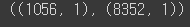
=> 여기서 index 값은 아래에서 train + test 값을 합쳐서 하나의 dataframe을 생성할 때 사용한다.
2) LSTNET 모델
1) sequnce Input conver 함수
def get_training_sequences(y, n_lookback):

    '''
    Split the time series into input sequences and output values. These are used for training the model.
    See Sections 3.1 and 3.8 in the LSTNet paper.
    Parameters:
    __________________________________
    y: np.array.
        Time series, array with shape (n_samples, n_targets) where n_samples is the length of the time
        series and n_targets is the number of time series.
    n_lookback: int.
        The number of past time steps used as input.
    Returns:
    __________________________________
    X: np.array.
        Input sequences, array with shape (n_samples - n_lookback, n_lookback, n_targets).
    Y: np.array.
        Output values, array with shape (n_samples - n_lookback, n_targets).
    '''

    X = np.zeros((y.shape[0], n_lookback, y.shape[1]))
    Y = np.zeros((y.shape[0], y.shape[1]))

    for i in range(n_lookback, y.shape[0]):

        X[i, :, :] = y[i - n_lookback: i, :]
        Y[i, :] = y[i, :]

    X = X[n_lookback:, :, :]
    Y = Y[n_lookback:, :]

    return X, Y
2) layer
class SkipGRU(tf.keras.layers.Layer):

    def __init__(self,
                 units,
                 p=1,
                 activation='relu',
                 return_sequences=False,
                 return_state=False,
                 **kwargs):

        '''
        Recurrent-skip layer, see Section 3.4 in the LSTNet paper.

        Parameters:
        __________________________________
        units: int.
            Number of hidden units of the GRU cell.
        p: int.
            Number of skipped hidden cells.
        activation: str, function.
            Activation function, see https://www.tensorflow.org/api_docs/python/tf/keras/activations.
        return_sequences: bool.
            Whether to return the last output or the full sequence.
        return_state: bool.
            Whether to return the last state in addition to the output.
        **kwargs: See https://www.tensorflow.org/api_docs/python/tf/keras/layers/GRUCell.
        '''

        if p < 1:
            raise ValueError('The number of skipped hidden cells cannot be less than 1.')

        self.units = units
        self.p = p
        self.return_sequences = return_sequences
        self.return_state = return_state
        self.timesteps = None
        self.cell = tf.keras.layers.GRUCell(units=units, activation=activation, **kwargs)

        super(SkipGRU, self).__init__()

    def build(self, input_shape):

        if self.timesteps is None:
            self.timesteps = input_shape[1]

            if self.p > self.timesteps:
                raise ValueError('The number of skipped hidden cells cannot be greater than the number of timesteps.')

    def call(self, inputs):

        '''
        Parameters:
        __________________________________
        inputs: tf.Tensor.
            Layer inputs, 2-dimensional tensor with shape (n_samples, filters) where n_samples is the batch size
            and filters is the number of channels of the convolutional layer.
        Returns:
        __________________________________
        outputs: tf.Tensor.
            Layer outputs, 2-dimensional tensor with shape (n_samples, units) if return_sequences == False,
            3-dimensional tensor with shape (n_samples, n_lookback, units) if return_sequences == True where
            n_samples is the batch size, n_lookback is the number of past time steps used as input and units
            is the number of hidden units of the GRU cell.
        states: tf.Tensor.
            Hidden states, 2-dimensional tensor with shape (n_samples, units) where n_samples is the batch size
            and units is the number of hidden units of the GRU cell.
        '''

        outputs = tf.TensorArray(
            element_shape=(inputs.shape[0], self.units),
            size=self.timesteps,
            dynamic_size=False,
            dtype=tf.float32,
            clear_after_read=False
        )

        states = tf.TensorArray(
            element_shape=(inputs.shape[0], self.units),
            size=self.timesteps,
            dynamic_size=False,
            dtype=tf.float32,
            clear_after_read=False
        )

        initial_states = tf.zeros(
            shape=(tf.shape(inputs)[0], self.units),
            dtype=tf.float32
        )

        for t in tf.range(self.timesteps):

            if t < self.p:
                output, state = self.cell(
                    inputs=inputs[:, t, :],
                    states=initial_states
                )

            else:
                output, state = self.cell(
                    inputs=inputs[:, t, :],
                    states=states.read(t - self.p)
                )

            outputs = outputs.write(index=t, value=output)
            states = states.write(index=t, value=state)

        outputs = tf.transpose(outputs.stack(), [1, 0, 2])
        states = tf.transpose(states.stack(), [1, 0, 2])

        if not self.return_sequences:
            outputs = outputs[:, -1, :]

        if self.return_state:
            states = states[:, -1, :]
            return outputs, states

        else:
            return outputs
3) model
## model check point
-> Sub class model은 아래의 sequence / functional 모델과는 다르게 checkpoint가 지정되지 않는다. 그러므로 아래와 같이 save class를 만들어서 사용한다.
## sequence / functional 모델의 경우 사용방법
## early stop / model_checkpoint
early_stopping = keras.callbacks.EarlyStopping(monitor='val_loss',patience=10)
model_checkpoint = keras.callbacks.ModelCheckpoint(
    filepath='./models/model_vgg16_trans/best_weights.h5',
    monitor='val_loss',
    save_best_only=True,
    verbose=1
)

batch_size=32

history_vgg16_trans = model_vgg16_trans.fit(train_generator, steps_per_epoch=len(X_train) // batch_size, epochs=100,
                              validation_data=val
### save class
class SaveModelH5(tf.keras.callbacks.Callback):
    def on_train_begin(self, logs=None):
         self.val_loss = []
    def on_epoch_end(self, epoch, logs=None):
        current_val_loss = logs.get("val_loss")
        self.val_loss.append(logs.get("val_loss"))
        if current_val_loss <= min(self.val_loss):
            print('Find lowest val_loss. Saving entire model.')
            self.model.save('model_save', save_format='tf') # < ----- Here
### model
class LSTNet():

    def __init__(self,
                 y,
                 forecast_period,
                 lookback_period,
                 filters=100,
                 kernel_size=3,
                 gru_units=100,
                 skip_gru_units=50,
                 skip=1,
                 lags=1,
                 dropout=0,
                 regularizer='L2',
                 regularization_factor=0.01):

        '''
        Implementation of multivariate time series forecasting model introduced in Lai, G., Chang, W. C., Yang, Y.,
        & Liu, H. (2018). Modeling Long- and Short-Term Temporal Patterns with Deep Neural Networks. In "The 41st
        International ACM SIGIR Conference on Research & Development in Information Retrieval" (SIGIR '18).
        Association for Computing Machinery, New York, NY, USA, 95–104.
        Parameters:
        __________________________________
        y: np.array.
            Time series, array with shape (n_samples, n_targets) where n_samples is the length of the time series
            and n_targets is the number of time series.
        forecast_period: int.
            Number of future time steps to forecast.
        lookback_period: int.
            Number of past time steps to use as input.
        filters: int.
            Number of filters (or channels) of the convolutional layer.
        kernel_size: int.
            Kernel size of the convolutional layer.
        gru_units: list.
            Hidden units of GRU layer.
        skip_gru_units: list.
            Hidden units of Skip GRU layer.
        skip: int.
            Number of skipped hidden cells in the Skip GRU layer.
        lags: int.
            Number of autoregressive lags.
        dropout: float.
            Dropout rate.
        regularizer: str.
            Regularizer, either 'L1', 'L2' or 'L1L2'.
        regularization_factor: float.
            Regularization factor.
        '''

        # Normalize the targets.
        y_min, y_max = np.min(y, axis=0), np.max(y, axis=0)
        y = (y - y_min) / (y_max - y_min)
        self.y_min = y_min
        self.y_max = y_max

        # Extract the input sequences and output values.
        self.X, self.Y = get_training_sequences(y, lookback_period)

        # Save the inputs.
        self.y = y
        self.n_samples = y.shape[0]
        self.n_targets = y.shape[1]
        self.n_lookback = lookback_period               #### n_step_in size
        self.n_forecast = forecast_period               #### n_step_out size

        # Build and save the model.
        self.model = build_fn(
            self.n_targets,
            self.n_lookback,
            filters,
            kernel_size,
            gru_units,
            skip_gru_units,
            skip,
            lags,
            dropout,
            regularizer,
            regularization_factor

        )


    def fit(self,
            loss='mse',
            monitor='val_loss',
            learning_rate=0.001,
            batch_size=32,
            epochs=100,
            validation_split=0,
            verbose=1,
            callbacks = []
            ):

        self.model.compile(
            optimizer=tf.keras.optimizers.Adam(learning_rate=learning_rate),
            loss=loss,
        )

        self.model.fit(
            x=self.X,
            y=self.Y,
            epochs=epochs,
            batch_size=batch_size,
            validation_split=validation_split,
            verbose=verbose,
            callbacks=callbacks,
        )

    def forecast(self, y):

        '''
        Generate the forecasts.

        Parameters:
        __________________________________
        y: np.array.
            Past values of the time series.
        Returns:
        __________________________________
        df: pd.DataFrame.
            Data frame including the actual values of the time series and the forecasts.
        '''

        # Normalize the targets.
        y = (y - self.y_min) / (self.y_max - self.y_min)

        # Generate the multi-step forecasts.
        x_pred = y[- self.n_lookback - 1: - 1, :].reshape(1, self.n_lookback, self.n_targets)   # Last observed input sequence.
        y_pred = y[-1:, :].reshape(1, 1, self.n_targets)                                        # Last observed target value.
        y_future = []                                                                           # Future target values.

        for i in range(self.n_forecast):

            # Feed the last forecast back to the model as an input.
            x_pred = np.append(x_pred[:, 1:, :], y_pred, axis=1)

            # Generate the next forecast.
            y_pred = self.model(x_pred).numpy().reshape(1, 1, self.n_targets)
            # print(f'y_pred : {y_pred}')

            # Save the forecast.
            y_future.append(y_pred.flatten().tolist())

        y_future = np.array(y_future)

        # Organize the forecasts in a data frame.
        columns = ['time_idx']
        columns.extend(['actual_' + str(i + 1) for i in range(self.n_targets)])
        columns.extend(['predicted_' + str(i + 1) for i in range(self.n_targets)])

        df = pd.DataFrame(columns=columns)
        df['time_idx'] = np.arange(self.n_samples + self.n_forecast)

        for i in range(self.n_targets):

            df['actual_' + str(i + 1)].iloc[: - self.n_forecast] = \
                self.y_min[i] + (self.y_max[i] - self.y_min[i]) * self.y[:, i]

            df['predicted_' + str(i + 1)].iloc[- self.n_forecast:] = \
                self.y_min[i] + (self.y_max[i] - self.y_min[i]) * y_future[:, i]

        # Return the data frame.
        return df.astype(float)


def build_fn(n_targets,
             n_lookback,
             filters,
             kernel_size,
             gru_units,
             skip_gru_units,
             skip,
             lags,
             dropout,
             regularizer,
             regularization_factor):

    '''
    Build the model, see Section 3 in the LSTNet paper.
    Parameters:
    __________________________________
    n_targets: int.
        Number of time series.
    n_lookback: int.
        Number of past time steps to use as input.
    filters: int.
        Number of filters (or channels) of the convolutional layer.
    kernel_size: int.
        Kernel size of the convolutional layer.
    gru_units: list.
        Hidden units of GRU layer.
    skip_gru_units: list.
        Hidden units of Skip GRU layer.
    skip: int.
        Number of skipped hidden cells in the Skip GRU layer.
    lags: int.
        Number of autoregressive lags.
    dropout: float.
        Dropout rate.
    regularizer: str.
        Regularizer, either 'L1', 'L2' or 'L1L2'.
    regularization_factor: float.
        Regularization factor.
    '''

    # Inputs.
    x = tf.keras.layers.Input(shape=(n_lookback, n_targets))

    # Convolutional component, see Section 3.2 in the LSTNet paper.
    c = tf.keras.layers.Conv1D(filters=filters, kernel_size=kernel_size, activation='relu')(x)
    c = tf.keras.layers.Dropout(rate=dropout)(c)

    # Recurrent component, see Section 3.3 in the LSTNet paper.
    r = tf.keras.layers.GRU(units=gru_units, activation='relu')(c)
    r = tf.keras.layers.Dropout(rate=dropout)(r)

    # Recurrent-skip component, see Section 3.4 in the LSTNet paper.
    s = SkipGRU(units=skip_gru_units, activation='relu', return_sequences=True)(c)
    s = tf.keras.layers.Dropout(rate=dropout)(s)
    s = tf.keras.layers.Lambda(function=lambda x: x[:, - skip:, :])(s)
    s = tf.keras.layers.Reshape(target_shape=(s.shape[1] * s.shape[2],))(s)
    d = tf.keras.layers.Concatenate(axis=1)([r, s])
    d = tf.keras.layers.Dense(units=n_targets, kernel_regularizer=kernel_regularizer(regularizer, regularization_factor))(d)

    # Autoregressive component, see Section 3.6 in the LSTNet paper.
    l = tf.keras.layers.Flatten()(x[:, - lags:, :])
    l = tf.keras.layers.Dense(units=n_targets, kernel_regularizer=kernel_regularizer(regularizer, regularization_factor))(l)

    # Outputs.
    y = tf.keras.layers.Add()([d, l])

    return tf.keras.models.Model(x, y)


def kernel_regularizer(regularizer, regularization_factor):

    '''
    Define the kernel regularizer.
    Parameters:
    __________________________________
    regularizer: str.
        Regularizer, either 'L1', 'L2' or 'L1L2'.
    regularization_factor: float.
        Regularization factor.
    '''

    if regularizer == 'L1':
        return tf.keras.regularizers.L1(l1=regularization_factor)

    elif regularizer == 'L2':
        return tf.keras.regularizers.L2(l2=regularization_factor)

    elif regularizer == 'L1L2':
        return tf.keras.regularizers.L1L2(l1=regularization_factor, l2=regularization_factor)

    else:
        raise ValueError('Undefined regularizer {}.'.format(regularizer))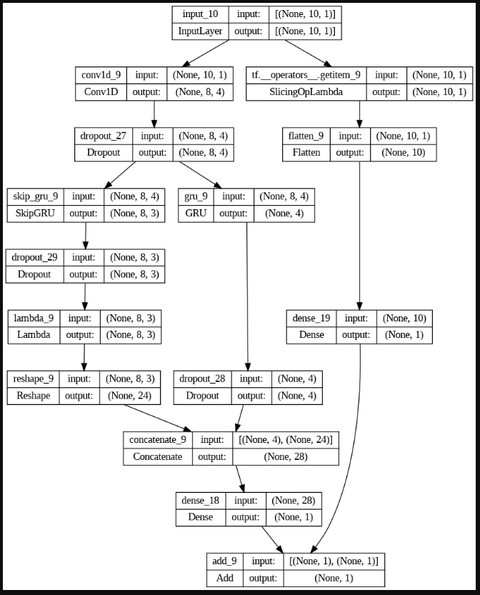
### 학습하기
forecast_period = 96

# Fit the model
model = LSTNet(
    y=y_train,
    forecast_period=forecast_period,
    lookback_period=24,
    kernel_size=3,
    filters=4,
    gru_units=4,
    skip_gru_units=3,
    skip=50,
    lags=100,
)

## model checkpoint
# save_model = SaveModelH5()
# callbacks=[save_model]

model.fit(
    loss='mse',
    learning_rate=0.01,
    batch_size=32,
    epochs=100,
    verbose=1,
    # callbacks = callbacks
)
=> 위에서 forecast_period 변수는 n_out_step으로 multi-step (예측 step)의 갯수를 의미하며,
lookback_period는 n_in_step으로 intput 설정 시 ( sample수 , timestep, feature수)로 들어가게 되는데 이때 timestep을 결정하는 값이다.
즉 앞의 lookback_period를 보고 forecast_period 개를 예측하겠다는 것을 의미한다.
학습시에는 Train / Label의 데이터는 아래와 같이 나눠진다.
X_train[0] =[1,2,3,4,5,6,7,8,10] => y_labe[0] =[11]
X_train[1] =[2,3,4,5,6,7,8,10,11] => y_labe[1] =[12]
X_train[2] =[3,4,5,6,7,8,10,11,12] => y_labe[2] =[13] 이런식으로 각 data와 label이 형성되며 이값을 학습 시킨다.
model예측을 수행하는 forcast는 y_labal이 한개씩 예측되므로 우리가 원하는 forecast_period 만큼 반복하여 수행된다.
        # Generate the multi-step forecasts.
        x_pred = y[- self.n_lookback - 1: - 1, :].reshape(1, self.n_lookback, self.n_targets)   # Last observed input sequence.
        y_pred = y[-1:, :].reshape(1, 1, self.n_targets)                                        # Last observed target value.
        y_future = []                                                                           # Future target values.

        for i in range(self.n_forecast):

            # Feed the last forecast back to the model as an input.
            x_pred = np.append(x_pred[:, 1:, :], y_pred, axis=1)

            # Generate the next forecast.
            y_pred = self.model(x_pred).numpy().reshape(1, 1, self.n_targets)
            # print(f'y_pred : {y_pred}')

            # Save the forecast.
            y_future.append(y_pred.flatten().tolist())

        y_future = np.array(y_future)
위의 코드에서 보면 x_pred 마지막 값에 y_pred값을 더한 마지막 관측치를 x_pred로 만들어서 self.model()에 넣어서 1step을 계산한다.

위의 그림에서 보면 조금 이해가 된다. 계속해서 y_pred값이 model로 부터 예측한 값으로 추가되어 x_pred가 되고 계속 계속 움직여 가며 forcast_period까지 예측이 된다.
### 예측하기
### predict
pred = model.forecast(y=y_train)

### index
pred_index = pd.to_datetime(y_train_idx + y_test_idx[:forecast_period])

### y_train[:-forecast_period]
actual_label = pred['actual_1'].values[:-forecast_period]
### y_test [:forecast_period]
y_test_new_ob = y_test[:forecast_period].reshape(-1)
### y_train[:-forecast_period] + y_test [:forecast_period] == label
label = np.concatenate((actual_label, y_test_new_ob), axis = 0)


### pred
prediction = pred['predicted_1'].values


### dataFrame
result_df = pd.DataFrame({
    'label' : label,
    'pred' : prediction,
}, index=pred_index)

result_df
### 그래프 그리기
from sklearn.metrics import mean_squared_error, r2_score, mean_absolute_error
mse = np.round(mean_squared_error( prediction[-forecast_period:] , y_test_new_ob ))
mae = np.round(mean_absolute_error( prediction[-forecast_period:] , y_test_new_ob ))
rmse = np.round(np.sqrt(mean_absolute_error( prediction[-forecast_period:] , y_test_new_ob )),2)
metric_df = pd.DataFrame([mse,mae,rmse], index=['MSE', 'MAE', 'RMSE']).T
display(metric_df)
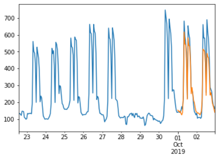
#### fig
fig, ax = plt.subplots()
fig.set_size_inches(25,7)
sns.lineplot(x=result_df.index ,y='label', data=result_df, ax=ax, label='label')
sns.lineplot(x=result_df.index ,y='pred', data=result_df, ax=ax, label='pred')
ax.grid()
ax.set(title=f'Prediction {forecast_period}th' )
ax.tick_params(axis='x', labelrotation=45)

뒷부분만 짤라서 보면 위와 같다. 너무많은 96step을 예측하면 생각보다 정확도가 낮은 것 같다.
조금씩 튜닝해가면서 방법을 찾아보아야 겠다.

'시계열분석_python' 카테고리의 다른 글
| [전력데이터 클러스터링]전력데이터 시간별 클러스터링_GMM (0) | 2023.04.21 |
|---|---|
| [SARIMAX]전력데이터 분석 ( ARIMA + Fourier 계절성 ) (0) | 2023.04.02 |
| [LSTNET]빌딩 전력 수요예측 (Functional 방법) (0) | 2023.03.26 |
| [SARIMA]빌딩 전력 시계열 모델 예측 (0) | 2023.03.23 |
| [서평이벤트 당첨_이지스퍼블리싱] 점프투 파이썬_라이브러리 예제편 (0) | 2022.05.27 |


