
| 일 | 월 | 화 | 수 | 목 | 금 | 토 |
|---|---|---|---|---|---|---|
| 1 | ||||||
| 2 | 3 | 4 | 5 | 6 | 7 | 8 |
| 9 | 10 | 11 | 12 | 13 | 14 | 15 |
| 16 | 17 | 18 | 19 | 20 | 21 | 22 |
| 23 | 24 | 25 | 26 | 27 | 28 | 29 |
| 30 |
- coding
- Instagrame clone
- 카트폴
- 앱개발
- 전국국밥
- 조코딩
- 강화학습 기초
- python
- 리액트네이티브
- 사이드프로젝트
- GYM
- 강화학습
- TeachagleMachine
- 데이터분석
- pandas
- FirebaseV9
- kaggle
- clone coding
- selenium
- ReactNative
- 클론코딩
- redux
- 머신러닝
- App
- JavaScript
- 딥러닝
- React
- Ros
- expo
- Reinforcement Learning
- Today
- Total
qcoding
[SARIMAX]전력데이터 분석 ( ARIMA + Fourier 계절성 ) 본문
** 아래의 글들을 참조하여 작성하였습니다.
https://robjhyndman.com/hyndsight/longseasonality/
Rob J Hyndman - Forecasting with long seasonal periods
robjhyndman.com
Forecasting time series with multiple seasonaliy by using auto_arima(SARIMAX) and Fourier terms
I am trying to forecast a time series in Python by using auto_arima and adding Fourier terms as exogenous features. The data come from kaggle's Store item demand forecasting challenge. It consists ...
stackoverflow.com
ARIMA : Trend(추세)를 반영한 모델
SARIMA : Sesoanl (계절성) 과 Trend(추세)를 반영한 모델
SARIMAX : SARIMA + exogeneous (외인성 인자)인 X를 더해서 계절성과 그외 요인인 인자를 반영한 모델
--> SARIMA의 경우 계절성 성분을 1개만 선택할 수 있으며, 이 계절성 성분은 일반적으로 m=200을 넘기면 메모리 문제가 발생한다.
--> 일반적인 실생활 데이터는 계절성 성분을 한개만 갖고 있지 않고, 주 / 월 / 연도별 패턴을 가지고 있으므로 단순히 SARIMA 문제로는 해결이 불가능하다. 이 떄 해결가능한 방법은 위의 블로그에서 말함 Fourier 방법이며, 아래의 식으로 나타낼 수 있다.

식에서 보면 SIN + COS 으로 이루어진 부분은 계절성을 담당하는 부분이며 N 에 해당하는 부분이 ARIMA에 대한 부분이다. 즉 Trend에 계절성 성분을 더하여 t 시점에 대한 값을 모델링 하는 것이다.
이 때 주의점은 SIN + COS 을 exogeneous (외인성 인자)로 넣어주게 되어 전체 모델은 SARIMA + X => SARIMAX 가 되는 데 이 때 Fourier값은 고정된 주기 m을 넣어주게 되므로 주기가 변할 수가 없다. 이 부분을 조심하면서 사용해야 할 것 같다.
### 데이터
import pandas as pd
import numpy as np
import seaborn as sns
import matplotlib.pyplot as plt
import tensorflow as tf
from tensorflow import keras

from sklearn.preprocessing import MinMaxScaler, OneHotEncoder
from sklearn.preprocessing import FunctionTransformer
from sklearn.metrics import mean_squared_error, r2_score, mean_absolute_error

import pandas as pd
from pmdarima.preprocessing import FourierFeaturizer
from pmdarima import auto_arima
import matplotlib.pyplot as plt

import calendar
import holidays

import pmdarima as pm
import pickle
import itertools

import statsmodels.api as sm
import os
### 데이터 전처리함수들
### data load
def chk_holiday(val):
    if val in kor_holidays:
        return 1
    else:
        return 0
def date_load(file_path):
df= pd.read_csv(file_path)
df = df.drop(columns=['Unnamed: 0'], axis=1)
return df# - 전력사용량 변수 결측치 발생 시 대체 알고리즘
# - pwr_qtly : t-1, t-2 시점의 평균치로 대체
def imp_pwr_qtly(dat, col):
for i in range(len(dat)):
k = dat.columns.get_loc(col)
if np.isnan(dat.iloc[i, k]) == True:
rep = dat.iloc[i - 1, k], dat.iloc[i - 2, k]
dat.iloc[i, k] = np.nanmean(rep)def feature_creating(df, date_column, group_hour):
if group_hour:
kor_holidays = list(holidays.KOR(years=range(2018,2020)).keys())
df = df.rename(columns={date_column : 'Date', 'load' : 'LOAD'})
df['Date'] = pd.to_datetime(df['Date'])
df['day_hour'] = df['Date'].dt.strftime('%Y-%m-%d %H')
df['day_hour'] = pd.to_datetime(df['day_hour'])
group = df.groupby(['day_hour'], as_index=False).mean()
group = group.rename(columns={"day_hour" : 'Date'})
group['year_day'] = group['Date'].dt.strftime('%Y-%m-%d')
group['year_day'] = pd.to_datetime(group['year_day'])
group['is_holiday'] = group['year_day'].map(lambda val: 1 if val in kor_holidays else 0)
group['weekday']=group['Date'].dt.weekday
group['workingday'] = np.where(group['weekday']>4, 0, 1)
cond_working= group['workingday'] == 1
cond_not_holiday = group['is_holiday'] !=1
group = group.loc[cond_working & cond_not_holiday]
return group
df = df.rename(columns={date_column : 'Date', 'load' : 'LOAD'})
df['Date'] = pd.to_datetime(df['Date'])
df['year']=df['Date'].dt.year
df['month']=df['Date'].dt.year
df['hour']=df['Date'].dt.hour
df['weekday']=df['Date'].dt.weekday
df['day'] = df['Date'].dt.day
df['workingday'] = np.where(df['weekday']>4, 0, 1)
df['day_hour'] = df['Date'].dt.strftime('%Y-%m-%d %H')
df['year_month']=df['Date'].dt.strftime('%Y-%m')
df['year_day'] = df['Date'].dt.strftime('%Y-%m-%d')
df['year_day'] = pd.to_datetime(df['year_day'])
kor_holidays = list(holidays.KOR(years=range(2016,2018)).keys())
df['is_holiday'] = df['year_day'].map(lambda val: 1 if val in kor_holidays else 0)
return dfdef data_split(df, test_start_date , indices_before, indices_after):
# set the number of indices before and after the control point to include in the train and test sets
### 15min 단위 데이터 일 경우
indices_before = indices_before # 31 -> 90일 전의 데이터 활용
indices_after = indices_after # 7일 -> 2일 후 데이터 예측
#### 여기서 data 나누면서 1~3월 / 4~6월 / 7~9월 / 10~12월 각각 점검 가능함
test_start_date = test_start_date
# get the index number of the test start date
test_start_index = df[df['Date'] == test_start_date].index[0]
# set the start and end indices for the train and test sets
## train idx
train_start_index = test_start_index - indices_before
train_end_index = test_start_index - 1
## test idx
test_end_index = test_start_index + indices_after
test_start_index = test_start_index
# split the data into train and test sets and select only the LOAD column
y_train = df.loc[train_start_index:train_end_index, ['LOAD']]
y_test = df.loc[test_start_index:test_end_index, ['LOAD']]
### 필요한 feature 정의
exogenous_features_num = []
# exogenous_features_num = ['humidity', '3hours_temp']
# exogenous_features_cat = [ 'weather' , 'is_holiday']
exogenous_features_cat = []
exogenous_features = exogenous_features_num + exogenous_features_cat
exogenous_train = df.loc[train_start_index:train_end_index,exogenous_features]
exogenous_test = df.loc[test_start_index:test_end_index,exogenous_features]
# exogenous_features = ["TEMP", "IS_WEEKDAY", "SKY_1", "SKY_2", "SKY_3", "SKY_4", "Day_1", "Day_2", "Day_3", "Day_4", "Day_5", "HOLIDAY"]
# convert DataFrame to Series
y_train = pd.Series(y_train["LOAD"], name='y_train')
y_test = pd.Series(y_test["LOAD"], name='y_test')
return y_train, y_test, exogenous_train, exogenous_test, exogenous_features, exogenous_features_num, exogenous_features_catdef preprocessing_feature(exogenous_train, exogenous_test, exogenous_features_num, exogenous_features_cat):
if exogenous_train.shape[1] == 0:
df_fil_train = pd.DataFrame()
df_fil_test = pd.DataFrame()
return df_fil_train , df_fil_test
df_train = exogenous_train
df_test = exogenous_test
x_num = exogenous_features_num
x_cat = exogenous_features_cat
## 수치형
min_max_scaler = MinMaxScaler(feature_range=(0, 1))
df_num_train = df_train[x_num]
df_num_test = df_test[x_num]
df_num_fil_train = min_max_scaler.fit_transform(df_num_train)
df_num_fil_test = min_max_scaler.transform(df_num_test)
df_num_fil_frame_train = pd.DataFrame(df_num_fil_train, columns=df_num_train.columns)
df_num_fil_frame_test = pd.DataFrame(df_num_fil_test, columns=df_num_test.columns)
# df_num_fil_frame.describe()
## 범주형
ohe = OneHotEncoder(sparse=False, handle_unknown='ignore')
df_cat_train = df_train[x_cat]
df_cat_test = df_test[x_cat]
df_cat_fil_train = ohe.fit_transform(df_cat_train.values.reshape(-1,len(df_cat_train.columns)))
df_cat_fil_test = ohe.transform(df_cat_test.values.reshape(-1,len(df_cat_test.columns)))
df_cat_fil_frame_train = pd.DataFrame(df_cat_fil_train, columns=ohe.get_feature_names_out ())
df_cat_fil_frame_test = pd.DataFrame(df_cat_fil_test, columns=ohe.get_feature_names_out ())
# df_cat_fil_frame.head()
## concat
index_train= df_train.index
df_fil_train = pd.concat([df_num_fil_frame_train, df_cat_fil_frame_train], axis=1)
df_fil_train=df_fil_train.set_index(index_train)
index_test= df_test.index
df_fil_test = pd.concat([df_num_fil_frame_test, df_cat_fil_frame_test], axis=1)
df_fil_test=df_fil_test.set_index(index_test)
return df_fil_train , df_fil_testdef log_transform(x):
# print(x)
return np.log(x + 1)
def preprocessing_label(y_train, y_test):
## train
scaler_load = FunctionTransformer(log_transform)
# scaler_load = MinMaxScaler(feature_range=(0,1))
y_train_scaled = scaler_load.fit_transform( y_train.values.reshape(-1,1) )
y_train_scaled = y_train_scaled.reshape(-1,)
## test
y_test_scaled = scaler_load.transform(y_test.values.reshape(-1,1))
y_test_scaled = y_test_scaled.reshape(-1,)
return y_train_scaled, y_test_scaled , scaler_loaddef exo_add_fourier(y_train_scaled, y_test_scaled, exogenous_train_scaled, exogenous_test):
### 연단위 주기 추가
# four_terms = FourierFeaturizer(365.25, 1) ## 연단위
# four_terms_day_1= FourierFeaturizer(12 * 1, 4) ## 일단위
four_terms_day= FourierFeaturizer(m=12*1, k=2) ## 일단위
# four_terms_week= FourierFeaturizer(m=24*1*7, k=2) ## 주 단위
# four_terms_month= FourierFeaturizer(m=24*1*30, k=2) ## 월 단위
# four_terms_year= FourierFeaturizer(24 * 365.25, 2) ## 연 단위
### Train
# _ ,exog_day_1 = four_terms_day.fit_transform(y_train_scaled)
_, exog_day_train = four_terms_day.fit_transform(y_train_scaled)
# _, exog_week_train = four_terms_week.fit_transform(y_train_scaled)
# _, exog_month_train = four_terms_month.fit_transform(y_train_scaled)
# _, exog_year_train = four_terms_year.fit_transform(y_train_scaled)
### Test
_, exog_day_test = four_terms_day.fit_transform(y_test_scaled)
# _, exog_week_test = four_terms_week.fit_transform(y_test_scaled)
# _, exog_month_test = four_terms_month.fit_transform(y_test_scaled)
# _, exog_year_test = four_terms_year.fit_transform(y_test_scaled)
# print(exog_day_train)
# print(exog_day_test)
# exog_four = pd.DataFrame()
# exog_four_train = pd.concat([exog_day_train, exog_week_train, exog_month_train, exog_year_train], axis=1) ###exog_month
# exog_four_test = pd.concat([exog_day_test, exog_week_test, exog_month_test, exog_year_test], axis=1)
exog_four_train = pd.concat([exog_day_train], axis=1) ###exog_month
exog_four_test = pd.concat([exog_day_test], axis=1)
# display(exog_four_train.head(3))
# display(exog_four_test.head(3))
## 기존의 exgenous feature add
## train
exogenous_train_scaled.reset_index(drop=True, inplace=True)
exog_four_train.reset_index(drop=True, inplace=True)
## test
exogenous_test.reset_index(drop=True, inplace=True)
exog_four_test.reset_index(drop=True, inplace=True)
exogenous_train_four_scaled = pd.concat([exogenous_train_scaled, exog_four_train], axis=1)
exogenous_test_four_scaled = pd.concat([exogenous_test, exog_four_test], axis=1)
return exogenous_train_four_scaled , exogenous_test_four_scaled### Main
## data load
file_path = './sarimax.csv'
df = date_load(file_path)
group_hour = True
df = feature_creating(df, 'Date', group_hour)
fig, ax = plt.subplots()
fig.set_size_inches(10,3)
sns.lineplot(x='Date', y='LOAD', data=df, ax=ax)
## 결측치처리
imp_pwr_qtly(df, 'LOAD')
df.isnull().sum()

## data split
test_start_date = '2018-11-29 00:00:00'
indices_before = ( 24 *1 ) * 90  # 31   -> 90일 전의 데이터 활용
indices_after = ( 24*1) * 7 - 1  # 7일 -> 2일 후 데이터 예측

y_train, y_test, exogenous_train, exogenous_test, exogenous_features, exogenous_features_num, exogenous_features_cat = data_split(df,test_start_date,indices_before,indices_after)
print(f'y_train : {y_train.shape} , y_test : {y_test.shape}, exogenous_train : {exogenous_train.shape}, exogenous_features : {len(exogenous_features)}')
## preprocessing
exogenous_train_scaled, exogenous_test_scaled= preprocessing_feature( exogenous_train ,exogenous_test, exogenous_features_num, exogenous_features_cat)
y_train_scaled, y_test_scaled , scaler_load = preprocessing_label(y_train, y_test)
exogenous_train_four_scaled, exogenous_test_four_scaled = exo_add_fourier(y_train_scaled, y_test_scaled, exogenous_train_scaled, exogenous_test_scaled)
print(f'exogenous_train_four_scaled : {exogenous_train_four_scaled.shape}, exogenous_test_four_scaled : {exogenous_test_four_scaled.shape} , y_train_scaled: {y_train_scaled.shape} , y_test_scaled: {y_test_scaled.shape}')
### SARIMAX 모델
### sarimax
from pmdarima.arima import ndiffs

kpss_diffs = ndiffs(y_train_scaled, alpha=0.05, test='kpss', max_d=6)
adf_diffs = ndiffs(y_train_scaled, alpha=0.05, test='adf', max_d=6)
n_diffs = max(adf_diffs, kpss_diffs)

print(f"추정된 차수 d = {n_diffs}")
model = pm.auto_arima(y=y_train_scaled, # df[0] = y_train
X=exogenous_train_four_scaled,
start_p=1, start_q=1,
max_p=5, max_q=5, # maximum p and q
start_P=1, start_Q=1,
max_P=3 ,max_Q=3,
m = 24, ## 여기서는 일주기 반영
d = n_diffs, # let model determine 'd'
D = 1,
max_D=2,
seasonal=False, # No Seasonality for standard ARIMA
trace=True, # logs
error_action='warn', # shows errors ('ignore' silences these)
suppress_warnings=True,
stepwise=True)
print(model.summary())
model.summary()
# save the order and seasonal_order
order = model.to_dict()['order']
seasonal_order = model.to_dict()['seasonal_order']
# save the order and seasonal_order to a file
#np.savez('LOAD_model_order.npz', order=order, seasonal_order=seasonal_order)
try:
save_path = './models/multiple_SARIMAX'
os.makedirs(f'{save_path}')
except:
pass
np.savez(f'{save_path}/model_order.npz', order=order, seasonal_order=seasonal_order)
### predic
# load the order and seasonal_order from the saved file
save_path = './models/multiple_SARIMAX'

Model_data = np.load(f'{save_path}/model_order.npz')
order = tuple(Model_data['order'])
seasonal_order = tuple(Model_data['seasonal_order'])


print(f'order : {order}   ,  seasonal_order : {seasonal_order}')

# ## MOEL FIT

model_sarima = pm.ARIMA(order=order, seasonal_order=seasonal_order)
model_sarima.fit(y=y_train_scaled, X=exogenous_train_four_scaled)

## PREDICTION
start = len(y_train_scaled)
end = len(y_train_scaled) + len(y_test_scaled) - 1
predictions = model_sarima.predict(n_periods=len(y_test_scaled[:-1]),X= exogenous_test_four_scaled.iloc[:-1,:], start=start, end=end, dynamic=False)


### data index 생성

# timestamp_str = datetime.now().strftime('%Y-%m-%d-%H-%M-%S')  ### production의 경우 현재 시간 이후로 생성
### development일 경우 train test이후로 생성
date_index = pd.date_range(test_start_date ,periods=len(predictions), freq='H')
# print(date_index)

#new_filename = f'LOAD_SARIMAX_{timestamp_str}.csv'
new_filename = f'{save_path}/output_load.csv'


# predictions_inv = scaler_load.inverse_transform(np.array(predictions).reshape(-1,1))
# y_test_inv = scaler_load.inverse_transform(np.array(y_test_scaled).reshape(-1,1))

# predictions_inv = predictions_inv.reshape(len(predictions_inv))
# y_test_inv = y_test_inv.reshape(len(y_test_inv))


predictions_inv = np.exp(predictions)
y_test_inv = np.exp(y_test_scaled)

# y_test_inv
pred = np.c_[predictions_inv, y_test_inv[:-1]]
df_pred = pd.DataFrame(pred, columns=['pred','label'] , index = date_index)
df_pred.to_csv(new_filename)

# save the model to a file
with open(f'{save_path}/model_order.pkl', 'wb') as f:
    pickle.dump(model, f)


import matplotlib as mpl
mpl.rcParams['text.color'] = 'black'


### plot
save_path = './models/multiple_SARIMAX'
result = pd.read_csv(f'{save_path}/output_load.csv')
result = result.rename(columns={"Unnamed: 0" : 'date'})
result['date'] = pd.to_datetime(result['date'])
result = result.set_index('date')


def MAPE(y_test, y_pred):
	return np.round(np.mean(np.abs((y_test - y_pred) / y_test)) * 100 )


mse = np.round(mean_squared_error( result['label'] , result['pred'] ))
mae = np.round(mean_absolute_error( result['label'] , result['pred'] ))
rmse = np.round(np.sqrt(mean_absolute_error( result['label'] , result['pred'] )),2)
mape = MAPE( result['label'] , result['pred'] )

metric_df = pd.DataFrame([mse,mae,rmse, mape], index=['MSE', 'MAE', 'RMSE','MAPE']).T
display(metric_df)

fig, axes = plt.subplots(nrows=2)
plt.subplots_adjust(hspace=0.5)
### 전체 train

date_train_index = pd.date_range(end=test_start_date ,periods=indices_before, freq='H')
date_train_index=date_train_index[-len(y_train_scaled):]
train_plot = pd.DataFrame({'label': y_train[-indices_before:].values}, index=date_train_index)


fig.set_size_inches(13,7)
fig.patch.set_facecolor('xkcd:white')

y_train[-indices_before:]

sns.lineplot(x=train_plot.index, y='label', data=train_plot, ax=axes[0], label='train_label') ## train_label
sns.lineplot(x=result.index, y='label', data=result, label='test_label', ax=axes[0]) ## test_label
sns.lineplot(x=result.index, y='pred', data=result, label='test_pred', ax=axes[0]) ## test_pred
axes[0].grid()
axes[0].legend()
axes[0].tick_params(axis='x', labelrotation=45)


sns.lineplot(x=result.index, y='label', data=result, label='label', ax=axes[1])
sns.lineplot(x=result.index, y='pred', data=result, label='pred', ax=axes[1])
axes[1].grid()
axes[1].legend()
axes[1].tick_params(axis='x', labelrotation=45)
### PIPE LINE
### pipe line
from pmdarima import pipeline
#from pmdarima import arima
from pmdarima import preprocessing as ppc

    # four_terms_day= FourierFeaturizer(m=24*1, k=2)  ## 일단위
    # four_terms_week= FourierFeaturizer(m=24*1*7, k=2)  ## 주 단위
    # four_terms_month= FourierFeaturizer(m=24*1*30, k=2)  ## 월 단위
    # four_terms_year= FourierFeaturizer(24 * 365.25, 2)  ## 연 단위


pipe = pipeline.Pipeline(
    [
     ("fourier_hour", ppc.FourierFeaturizer(m=(12*1 * 1), k=2)),
     ("fourier_day", ppc.FourierFeaturizer(m=(24*1 * 1), k=2)),
     ("fourier_week", ppc.FourierFeaturizer(m=(24*1* 7), k=2)),
    #  ("fourier_month", ppc.FourierFeaturizer(m=(24*1*365.25/12), k=2)),
    #  ("fourier_year", ppc.FourierFeaturizer(m=(24*1*365.25), k=2)),
     ("arima", pm.AutoARIMA(#exogenous = exogenous_train[exogenous_features],
                               test='adf', # use adftest to find optimal 'd'
                               max_p=3, max_q=3, # maximum p and q
                               m=96, # frequency of series (if m==1, seasonal is set to FALSE automatically)
                               d=1,# let model determine 'd'
                               seasonal=False, # No Seasonality for standard ARIMA
                               trace=True, #logs
                               error_action='warn', #shows errors ('ignore' silences these)
                               suppress_warnings=True,
                               stepwise=True))
    ])

### fit
pipe.fit(y_train_scaled)


### save
## 모델 저장
# save the model to a file
try:
    save_path = './models/multiple_SARIMAX_pipe'
    os.makedirs(f'{save_path}')
except:
    pass

with open(f'{save_path}/model.pkl', 'wb') as f:
    pickle.dump(pipe, f)
### PIPE LINE 예측하기
### model load
save_path = './models/multiple_SARIMAX_pipe'
with open(f'{save_path}/model.pkl', 'rb') as f:
    load_pipe_model = pickle.load(f)


# max_p = load_pipe_model.steps[-1][-1].max_p
# max_q = load_pipe_model.steps[-1][-1].max_q
# d_ = load_pipe_model.steps[-1][-1].d

# PREDICTION
### fit 하면 다시 학습시작
# load_pipe_model.fit(y_train_scaled)

start = len(y_train_scaled)
end = len(y_train_scaled) + len(y_test_scaled) - 1
predictions = load_pipe_model.predict(len(y_test_scaled[:-1]))

# y_predict_pipe = pd.DataFrame(y_predict_pipe,index = y_test.index,columns=['Pipe Prediction'])

### data index 생성

# timestamp_str = datetime.now().strftime('%Y-%m-%d-%H-%M-%S')  ### production의 경우 현재 시간 이후로 생성
### development일 경우 train test이후로 생성
date_index = pd.date_range(test_start_date ,periods=len(predictions), freq='H')
# print(date_index)

#new_filename = f'LOAD_SARIMAX_{timestamp_str}.csv'
new_filename = f'{save_path}/output_load_pip.csv'


predictions_inv = np.exp(predictions)
y_test_inv = np.exp(y_test_scaled)

# y_test_inv
pred = np.c_[predictions_inv, y_test_inv[:-1]]
df_pred = pd.DataFrame(pred, columns=['pred','label'] , index = date_index)
df_pred.to_csv(new_filename)

### plot
save_path = './models/multiple_SARIMAX_pipe'
result = pd.read_csv(f'{save_path}/output_load_pip.csv')
result = result.rename(columns={"Unnamed: 0" : 'date'})
result['date'] = pd.to_datetime(result['date'])
result = result.set_index('date')


def MAPE(y_test, y_pred):
	return np.round(np.mean(np.abs((y_test - y_pred) / y_test)) * 100 )


mse = np.round(mean_squared_error( result['label'] , result['pred'] ))
mae = np.round(mean_absolute_error( result['label'] , result['pred'] ))
rmse = np.round(np.sqrt(mean_absolute_error( result['label'] , result['pred'] )),2)
mape = MAPE( result['label'] , result['pred'] )

metric_df = pd.DataFrame([mse,mae,rmse, mape], index=['MSE', 'MAE', 'RMSE','MAPE']).T
display(metric_df)


fig, axes = plt.subplots(nrows=2)
plt.subplots_adjust(hspace=0.5)
### 전체 train

date_train_index = pd.date_range(end=test_start_date ,periods=indices_before, freq='H')
date_train_index=date_train_index[-len(y_train_scaled):]
train_plot = pd.DataFrame({'label': y_train[-indices_before:].values}, index=date_train_index)


fig.set_size_inches(13,7)
fig.patch.set_facecolor('xkcd:white')

y_train[-indices_before:]

sns.lineplot(x=train_plot.index, y='label', data=train_plot, ax=axes[0], label='train_label') ## train_label
sns.lineplot(x=result.index, y='label', data=result, label='test_label', ax=axes[0]) ## test_label
sns.lineplot(x=result.index, y='pred', data=result, label='test_pred', ax=axes[0]) ## test_pred
axes[0].grid()
axes[0].legend()
axes[0].tick_params(axis='x', labelrotation=45)


sns.lineplot(x=result.index, y='label', data=result, label='label', ax=axes[1])
sns.lineplot(x=result.index, y='pred', data=result, label='pred', ax=axes[1])
axes[1].grid()
axes[1].legend()
axes[1].tick_params(axis='x', labelrotation=45)
## 결과정리
코드는 위와 같이 auto arima 또는 pipeline으로 구축하여 사용한다.
1) m (주기) = 12 일때, 12개의 계절성을 갖는다고 생각
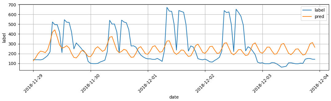
위의 그림처럼 12시간의 작은 주기가 반영되어 전체 데이터의 주기를 반영하지 못한다. 주기를 좀더 늘려서 일주기를 반영할 수 있게 해본다.
2) m (주기) =12 (12시간) / 24 (일일) / 24 *7 (주간)

위의 같이 시간 / 일 / 주간을 다 반영한 주기를 넣으면
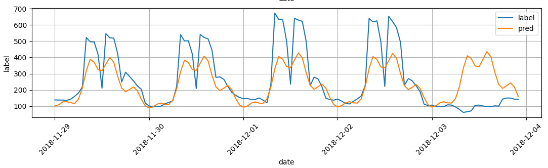
일 주기내에 있는 시간 주기를 만족시키는 것을 볼 수 있으며, 일별로 증가 추세를 맞출 수 있다. 그러나 아직 전체적인 크기는 맞출 수 없으며 12월 3일 처럼 일반적인 패턴을 따라 가지 않은 경우는 맞출 수 없는 것을 볼 수 있다. 이것이 위에 말한 고정된 주기성을 의미한다.
3) m (주기) =12 (12시간) / 24 (일일) / 24 *7 (주간) / 24 * 365.25/12 (월)


위에는 월주기를 추가해서 반영한 것을 보여준다. 월주기를 반영해도 데이터가 크게 달라지지 않은 것 같다. 아마 이 데이터는 2018년부터 2020년 까지의 1시간 별 데이터로 연주기까지 반영해 주어야 값이 맞을 것 같다.
4) m (주기) =12 (12시간) / 24 (일일) / 24 *7 (주간) / 24 * 365.25/12 (월) / 24 * 365.25 (연)


위의 모든 주기를 다 반영하면 3일 정도까지의 예측은 잘 맞지만 그외에는 더 많은 주기가 반영되어 값이 커지는 것을 볼 수 있다. 최종적으로는 이 값이 가장 좋지만 장기적인 예측 보다는 좀더 짧은 주기의 예측에 적합할 것 같다.
'시계열분석_python' 카테고리의 다른 글
| [전력데이터 클러스터링]전력데이터 시간별 클러스터링_GMM (0) | 2023.04.21 |
|---|---|
| [LSTNET]빌딩 전력 수요예측 (Functional 방법) (0) | 2023.03.26 |
| [LSTNET] 빌딩전력예측 딥러닝 (0) | 2023.03.26 |
| [SARIMA]빌딩 전력 시계열 모델 예측 (0) | 2023.03.23 |
| [서평이벤트 당첨_이지스퍼블리싱] 점프투 파이썬_라이브러리 예제편 (0) | 2022.05.27 |


